Three Dimensional Shapes and Shading

Jan 24, 2021 · 13 min read · python vector 3D shading cross product mathplotlib ·

Three dimensional objects are not easy to represent on a 2D surface such as a page or screen. In this article, inspired by chapter 3 of Math for Programmers book, we look at the cross product of two 3D-vectors and representing the surface of any 3D object as a collection of triangles. The cross product can be used to determine the direction of a triangle and this can be used to determine if the triangle is visible and the level of shading.

These are my notes on the book Math for Programmers by Paul Orland.

2D vectors and vector arithmetic
Two Dimensional shapes
Three Dimensional Vectors and Dot Product
Three Dimensional Shapes and Shading

Cross product

The cross product of two vectors v and u (v × u), is a vector that is perpendicular to both v and u, and therefore normal to the plane containing them. The magnitude of the cross product vector equals the area of a parallelogram with the vectors for sides. The direction of the vector of the cross product obeys the right-hand rule.

The orientation of the three axes in three-dimensional space can have two possible orientations. The right-hand rule is a common mnemonic for understanding orientation of axes in three-dimensional space. One can see this by pointing the right index finger along the positive x-axis and curl the remaining fingers toward the positive y-axis, the thumb tells you the direction of the positive z-axis.

The formula to calculate the cross product seems a little complex at first. It is easy to write a python function to calculate the cross product.

$$ \begin{gathered} vector \ u = (u_x, \ u_y, \ u_z) \\\ vector \ v = (v_x, \ v_y, \ v_z) \end{gathered} $$

$$ u \ {\times} \ v = (u_yv_z - u_zv_y, \ u_zv_x - u_xv_z , \ u_xv_y - u_yv_x) $$

Adding color to the x,y,z coordinates makes it easier to see that the resultant coordinate is made from the difference of the products of the other two coordinates. For example the cross product x coordinate is the difference of the y*z and z*y of the vectors. Note that cross product is noncommutative in that u x v is not equal to v x u.

$$ vector \ u = (u_{\color{aqua}x}, \ u_{\color{fuchsia}y}, \ u_{\color{olive}z}), \\\ vector \ v = (v_{\color{aqua}x}, \ v_{\color{fuchsia}y}, \ v_{\color{olive}z}) $$

$$ u \ {\times} \ v = (u_{\color{fuchsia}y}v_{\color{olive}z} - u_{\color{olive}z}v_{\color{fuchsia}y}, \ u_{\color{olive}z}v_{\color{aqua}x} - u_{\color{aqua}x}v_{\color{olive}z} , \ u_{\color{aqua}x}v_{\color{fuchsia}y} - u_{\color{fuchsia}y}v_{\color{aqua}x}) $$

$$ u \ {\times} \ v \neq v \ {\times} \ u $$

 1def cross(u, v):
 2    ux,uy,uz = u
 3    vx,vy,vz = v
 4    return (uy*vz - uz*vy, uz*vx - ux*vz, ux*vy - uy*vx)
 5
 6print(cross((3, 4, 5), (4, 4, 4)))
 7print(cross((4, 4, 4), (3, 4, 5)))
 8
 9"""
10(-4, 8, -4)
11(4, -8, 4)
12"""

 1def plot_axes(ax):
 2    ax.plot((-4, 4), (0, 0), (0, 0), color="grey")
 3    ax.plot((0, 0), (-4, 4), (0, 0), color="grey")
 4    ax.plot((0, 0), (0, 0), (-4, 4), color="grey")
 5
 6
 7def plot_vector(ax, v, c):
 8    ax.plot((0, v[0]), (0, v[1]), (0, v[2]), color=c)
 9
10
11def update_axis(ax, v1, v2):
12    plot_axes(ax)
13    plot_vector(ax, v1, "blue")
14    plot_vector(ax, v2, "red")
15    vx = cross(v1, v2)
16    plot_vector(ax, vx, "cyan")
17    ax.set_title(f"\n{v1} x {v2} \ncross product = {vx}", fontsize=10)
18
19
20fig, axs = plt.subplots(
21    2, 3, figsize=(10, 8), facecolor=plt.cm.Blues(0.2), subplot_kw={"projection": "3d"}
22)
23fig.suptitle(
24    f"Cross product of two 3D-vectors",
25    fontsize=18,
26    fontweight="bold",
27)
28
29for i, ax in enumerate(axs.flatten()):
30    ax.set_facecolor(plt.cm.Blues(0.1))
31    ax.set_xlim(-7, 5)
32    ax.set_ylim(-5, 5)
33    ax.set_zlim(-6, 10)
34    ax.set_xlabel("x-axis")
35    ax.set_ylabel("y-axis")
36    ax.set_zlabel("z-axis")
37
38u = (3, 4, 5)
39v = (4, 4, 4)
40update_axis(axs[0][0], u, v)
41update_axis(axs[0][1], v, u)
42update_axis(axs[1][0], u, v)
43update_axis(axs[1][1], v, u)
44
45u = (2, 2, 0)
46v = (0, 4, 0)
47update_axis(axs[0][2], u, v)
48update_axis(axs[1][2], v, u)
49
50for ax in [axs[1][0], axs[1][1], axs[1][2]]:
51    ax.view_init(azim=-80)
52
53fig.tight_layout(pad=2.0)
54plt.show()

Cross product of 3D vectors viewed from two angles

Length of Cross Product

The magnitude (length) of the cross product is equal to the area of the parallelogram formed by the two vectors. The cross product of parallel vectors is zero as is the cross product of opposite vectors. The magnitude of the cross product of two vectors is at a maximum when those vectors are at 90⁰ to each other.

 1def plot_axes(ax):
 2    ax.plot((-4, 4), (0, 0), (0, 0), color="grey")
 3    ax.plot((0, 0), (-4, 4), (0, 0), color="grey")
 4    ax.plot((0, 0), (0, 0), (-4, 4), color="grey")
 5
 6
 7def plot_vector(ax, v, c):
 8    ax.plot((0, v[0]), (0, v[1]), (0, v[2]), color=c)
 9
10
11def update_axis(ax, v1, v2):
12    plot_axes(ax)
13    plot_vector(ax, v1, "blue")
14    plot_vector(ax, v2, "red")
15    vx = cross(v1, v2)
16    plot_vector(ax, vx, "cyan")
17    ax.set_title(
18        f"\n{v1} x {v2} \nlength cross product = {vector_length(vx):.1F}", fontsize=10
19    )
20
21
22fig, axs = plt.subplots(
23    2, 3, figsize=(10, 8), facecolor=plt.cm.Blues(0.2), subplot_kw={"projection": "3d"}
24)
25fig.suptitle(
26    f"Length of cross product of two 3D-vectors",
27    fontsize=18,
28    fontweight="bold",
29)
30
31for i, ax in enumerate(axs.flatten()):
32    ax.set_facecolor(plt.cm.Blues(0.1))
33    ax.set_xlim(-7, 5)
34    ax.set_ylim(-5, 5)
35    ax.set_zlim(-6, 10)
36    ax.set_xlabel("x-axis")
37    ax.set_ylabel("y-axis")
38    ax.set_zlabel("z-axis")
39
40update_axis(axs[0][0], (3, 0, 0), (3, 0, 0))
41update_axis(axs[0][1], (3, 0, 0), (2, 2, 0))
42update_axis(axs[0][2], (3, 0, 0), (1, 3, 0))
43update_axis(axs[1][0], (3, 0, 0), (0, 3, 0))
44update_axis(axs[1][1], (3, 0, 0), (-2, 2, 0))
45update_axis(axs[1][2], (3, 0, 0), (-3, 0, 0))
46
47plt.show()
48
49publish_png_image(fig, "length-of-cross-product-3d-vector.png")

Length of cross product is equal to parallelogram area

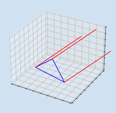
Triangle composed of 3 vectors

A triangle is composed of three sides or three vectors. Each vector is composed of two sets of coordinates, a start and an end. To form a triangle the three vectors must be connected so the start/end of one vector must match the start/end of another vector.

 1def add_vectors(*v):
 2    return tuple(sum(x) for x in zip(*v))
 3
 4
 5def subtract_vectors(v1, v2):
 6    return tuple(x[0] - x[1] for x in zip(v1, v2))
 7
 8
 9print(subtract_vectors((2, 3, 4), (0, 0, 0)))
10print(subtract_vectors((2, 3, 4), (4, 4, 4)))
11"""
12(2, 3, 4)
13(-2, -1, 0)
14"""

 1def plot_axes(ax):
 2    ax.plot((-3, 3), (0, 0), (0, 0), color="grey")
 3    ax.plot((0, 0), (-3, 3), (0, 0), color="grey")
 4    ax.plot((0, 0), (0, 0), (-3, 3), color="grey")
 5
 6
 7def plot_vector(ax, v1, v2, c):
 8    ax.plot((v1[0], v2[0]), (v1[1], v2[1]), (v1[2], v2[2]), color=c)
 9
10
11def update_axis(ax, *vectors):
12    for v in vectors:
13        plot_vector(ax, v[0], v[1], "blue")
14
15
16fig, axs = plt.subplots(
17    1, 3, figsize=(10, 4), facecolor=plt.cm.Blues(0.2), subplot_kw={"projection": "3d"}
18)
19fig.suptitle(
20    f"Cross Product on a Triangle",
21    fontsize=18,
22    fontweight="bold",
23)
24
25titles = ["Vectors", "Triangle", "Cross Product"]
26for i, ax in enumerate(axs.flatten()):
27    ax.set_facecolor(plt.cm.Blues(0.1))
28    ax.set_xlim(-3, 3)
29    ax.set_ylim(-3, 3)
30    ax.set_zlim(-3, 3)
31    ax.set_xlabel("x-axis")
32    ax.set_ylabel("y-axis")
33    ax.set_zlabel("z-axis")
34    ax.set_title(titles[i])
35    plot_axes(ax)
36
37# triangle
38t = ((2, 0, 0), (0, 2, 0), (0, 0, 2))
39orig = (0, 0, 0)
40cp = add_vectors(
41    t[0], cross(subtract_vectors(t[1], t[0]), subtract_vectors(t[2], t[0]))
42)
43
44update_axis(axs[0], (orig, t[0]), (orig, t[1]), (orig, t[2]))
45update_axis(axs[1], (t[0], t[1]), (t[0], t[2]), (t[1], t[2]))
46update_axis(axs[2], (t[0], t[1]), (t[0], t[2]), (t[1], t[2]))
47plot_vector(ax, t[0], cp, "Red")
48
49plt.show()

Use of Cross Product to determine the outward side of a triangle

Shading

shading refers to the process of altering the color of an object based on the source of light and the viewing perspective as well as the angle of the light and the angle of the object surface to the viewer. Ultimately the 3D objects are displayed on the 2D screen and based on calculations using properties like cross product and projecting the visible surfaces onto a 2D surface, the 3D object is presented for viewing.

The vertices of a shape can be plotted to display the shape or the plot_wireframe function from matplotlib can be used. Similarly, instead of calculating the surface and shading of an object, the plot_surface function is used. The following code plots a triangle using vertices as well as the plot_wireframe and plot_surface functions.

 1def plot_axes(ax):
 2    ax.plot((-2, 2), (0, 0), (0, 0), color="grey")
 3    ax.plot((0, 0), (-2, 2), (0, 0), color="grey")
 4    ax.plot((0, 0), (0, 0), (-2, 2), color="grey")
 5
 6
 7def plot_vector(ax, v1, v2, c):
 8    ax.plot((v1[0], v2[0]), (v1[1], v2[1]), (v1[2], v2[2]), color=c)
 9
10
11def plot_polygon(ax, *v):
12    for i in range(len(v)):
13        j = (i + 1) % len(v)
14        plot_vector(ax, v[i], v[j], "Blue")
15
16
17fig, axs = plt.subplots(
18    1, 3, figsize=(10, 4), facecolor=plt.cm.Blues(0.2), subplot_kw={"projection": "3d"}
19)
20fig.suptitle(
21    f"Plotting a triangle in 3D",
22    fontsize=18,
23    fontweight="bold",
24)
25
26for i, ax in enumerate(axs.flatten()):
27    ax.set_facecolor(plt.cm.Blues(0.1))
28    ax.set_xlim(-1, 3)
29    ax.set_ylim(-1, 3)
30    ax.set_zlim(-1, 3)
31    ax.set_xlabel("x-axis")
32    ax.set_ylabel("y-axis")
33    ax.set_zlabel("z-axis")
34    plot_axes(ax)
35
36# triangle vertices
37triangle = [(0, 2, 0), (2, 2, 0), (0, 2, 2)]
38plot_polygon(axs[0], *triangle)
39axs[0].set_title("Vertices")
40
41x = np.array([[0, 2], [0, 0]])
42y = np.array([[2, 2], [2, 2]])
43z = np.array([[0, 0], [0, 2]])
44axs[1].plot_wireframe(x, y, z, color="Blue")
45axs[1].set_title("plot_wireframe")
46
47axs[2].plot_surface(x, y, z, color="Blue")
48axs[2].set_title("plot_surface")
49
50plt.show()

Plot triangle using plot_wireframe and plot_surface functions

 1def plot_vector(ax, v1, v2, c):
 2    ax.plot((v1[0], v2[0]), (v1[1], v2[1]), (v1[2], v2[2]), color=c)
 3
 4
 5def plot_polygon(ax, *v):
 6    for i in range(len(v)):
 7        j = (i + 1) % len(v)
 8        plot_vector(ax, v[i], v[j], "Blue")
 9
10
11fig, axs = plt.subplots(
12    1, 3, figsize=(10, 4), facecolor=plt.cm.Blues(0.2), subplot_kw={"projection": "3d"}
13)
14fig.suptitle(
15    f"Vertices in a side",
16    fontsize=18,
17    fontweight="bold",
18)
19
20for i, ax in enumerate(axs.flatten()):
21    ax.set_facecolor(plt.cm.Blues(0.1))
22    ax.set_xlim(-1, 3)
23    ax.set_ylim(-1, 3)
24    ax.set_zlim(-1, 3)
25    ax.set_xlabel("x-axis")
26    ax.set_ylabel("y-axis")
27    ax.set_zlabel("z-axis")
28    ax.set_title(titles[i])
29
30square = [(2, 2, 2), (0, 2, 2), (0, 2, 0), (2, 2, 0)]
31plot_polygon(axs[0], *square)
32axs[0].set_title("Vertices")
33
34x = np.array([[2, 0], [2, 0]])
35y = np.array([[2, 2], [2, 2]])
36z = np.array([[2, 2], [0, 0]])
37axs[1].plot_wireframe(x, y, z, color="Blue")
38axs[1].set_title("plot_wireframe")
39
40axs[2].plot_surface(x, y, z, color="Blue")
41axs[2].set_title("plot_surface")
42
43plt.show()

Plot square using plot_wireframe and plot_surface functions

Cube

Plotting a 3D object using vertices and plotting segments and faces can get complicated without functions like plot_wireframe and plot_surface. A NumPy 2-dimensional array is used for the x,y and z coordinates. plot_surface has a number of parameters that can be used to customise the rendered object such as lightsource as used in the third plot.

 1fig, (ax1, ax2, ax3) = plt.subplots(
 2    1, 3, figsize=(10, 4), facecolor=plt.cm.Blues(0.2), subplot_kw={"projection": "3d"}
 3)
 4fig.suptitle(
 5    f"Cube",
 6    fontsize=18,
 7    fontweight="bold",
 8)
 9
10for i, ax in enumerate([ax1, ax2, ax3]):
11    ax.set_facecolor(plt.cm.Blues(0.1))
12    ax.set_xlim(-1, 3)
13    ax.set_ylim(-1, 3)
14    ax.set_zlim(-1, 3)
15    ax.set_xlabel("x-axis")
16    ax.set_ylabel("y-axis")
17    ax.set_zlabel("z-axis")
18
19x = np.array(
20    [
21        [2, 0, 0, 2, 2],
22        [2, 0, 0, 2, 2],
23        [0, 2, 2, 0, 0],
24        [0, 2, 2, 0, 0],
25        [2, 0, 0, 2, 2],
26    ]
27)
28
29y = np.array(
30    [
31        [2, 2, 0, 0, 2],
32        [2, 2, 0, 0, 2],
33        [0, 0, 2, 2, 0],
34        [0, 0, 2, 2, 0],
35        [2, 2, 0, 0, 2],
36    ]
37)
38
39z = np.array(
40    [
41        [2, 2, 2, 2, 2],
42        [0, 0, 0, 0, 0],
43        [0, 0, 0, 0, 0],
44        [2, 2, 2, 2, 2],
45        [2, 2, 2, 2, 2],
46    ]
47)
48
49ax1.set_title("Wireframe")
50ax1.plot_wireframe(x, y, z)
51
52ax2.set_title("Surface")
53ax2.plot_surface(x, y, z)
54
55ax3.set_title("Light Source")
56ls = matplotlib.colors.LightSource(4, -4, 4)
57ax3.plot_surface(x, y, z, lightsource=ls)
58
59plt.show()

Plot cube using plot_wireframe and plot_surface functions

Sphere

Like a circle or a curved line in 2D-space can be represented by a sequence of small straight lines, a curved surface in 3D-space can be represented by a collection of small triangles. The higher the number of segments the more curved the sphere will appear.

 1def create_sphere(segments):
 2    u = np.linspace(0, 2 * np.pi, segments)
 3    v = np.linspace(0, np.pi, segments)
 4    x = 20 * np.outer(np.cos(u), np.sin(v))
 5    y = 20 * np.outer(np.sin(u), np.sin(v))
 6    z = 20 * np.outer(np.ones(np.size(u)), np.cos(v))
 7    return (x, y, z)
 8
 9
10fig, (ax1, ax2, ax3) = plt.subplots(
11    1, 3, figsize=(10, 4), facecolor=plt.cm.Blues(0.2), subplot_kw={"projection": "3d"}
12)
13fig.suptitle(
14    f"Sphere Wireframes",
15    fontsize=18,
16    fontweight="bold",
17)
18
19for i, ax in enumerate([ax1, ax2, ax3]):
20    ax.set_facecolor(plt.cm.Blues(0.1))
21    ax.set_xlim(-25, 25)
22    ax.set_ylim(-25, 25)
23    ax.set_zlim(-25, 25)
24    ax.set_xlabel("x-axis")
25    ax.set_ylabel("y-axis")
26    ax.set_zlabel("z-axis")
27    n = 5 * i + 10
28    ax.set_title(f"segments: {n}")
29    (x, y, z) = create_sphere(n)
30    ax.plot_wireframe(x, y, z)
31
32plt.show()

Plot sphere using plot_wireframe with increasing numbers of segments

Plot sphere wireframe with increasing numbers of segments

 1def create_sphere(segments):
 2    u = np.linspace(0, 2 * np.pi, segments)
 3    v = np.linspace(0, np.pi, segments)
 4    x = 20 * np.outer(np.cos(u), np.sin(v))
 5    y = 20 * np.outer(np.sin(u), np.sin(v))
 6    z = 20 * np.outer(np.ones(np.size(u)), np.cos(v))
 7    return (x, y, z)
 8
 9
10fig, axs = plt.subplots(
11    2, 3, figsize=(10, 8), facecolor=plt.cm.Blues(0.2), subplot_kw={"projection": "3d"}
12)
13fig.suptitle(
14    f"Sphere composed with increasing number of segments",
15    fontsize=18,
16    fontweight="bold",
17)
18
19for i, ax in enumerate(axs.flatten()):
20    ax.set_facecolor(plt.cm.Blues(0.1))
21    ax.set_xlim(-25, 25)
22    ax.set_ylim(-25, 25)
23    ax.set_zlim(-25, 25)
24    ax.set_xlabel("x-axis")
25    ax.set_ylabel("y-axis")
26    ax.set_zlabel("z-axis")
27    n = (10 * i) + 10
28    ax.set_title(f"segments: {n}")
29    (x, y, z) = create_sphere(n)
30    ax.plot_surface(x, y, z)
31
32plt.show()

Plot sphere using plot_surface with increasing numbers of segments

Plot sphere surface with increasing numbers of segments

Plot sphere with decreasing transparency

Torus

A Torus is a geometric surface generated by revolving a circle in 3-D space about an axis that is coplanar with the circle. A real-world objects that approximate a torus of revolution is an inner tube and an example of a solid torus is a ring doughnut or bagel.

 1def create_torus(segments):
 2    u = np.linspace(0, 2 * np.pi, segments)
 3    v = np.linspace(0, 2 * np.pi, segments)
 4    u, v = np.meshgrid(u, v)
 5    a,b = 5,9
 6    x = (b + a * np.cos(u)) * np.cos(v)
 7    y = (b + a * np.cos(u)) * np.sin(v)
 8    z = a * np.sin(u)
 9    return (x, y, z)
10
11
12fig, (ax1, ax2) = plt.subplots(
13    1, 2, figsize=(10, 5), facecolor=plt.cm.Blues(0.2), subplot_kw={"projection": "3d"}
14)
15fig.suptitle(
16    f"Torus",
17    fontsize=18,
18    fontweight="bold",
19)
20
21(x, y, z) = create_torus(50)
22
23for i, ax in enumerate([ax1, ax2]):
24    ax.set_facecolor(plt.cm.Blues(0.1))
25    ax.set_xlim(-14, 14)
26    ax.set_ylim(-14, 14)
27    ax.set_zlim(-14, 14)
28    ax.set_xlabel("x-axis")
29    ax.set_ylabel("y-axis")
30    ax.set_zlabel("z-axis")
31
32ax1.set_title(f"wireframe")
33ax1.plot_wireframe(x, y, z)
34
35ax2.set_title(f"surface")
36ax2.plot_surface(x, y, z)
37
38plt.show()

Plot torus

Conclusion

The cross product of two vectors is a vector that is perpendicular to both vectors. The magnitude of the cross product vector equals the area of a parallelogram with the vectors for sides. The direction of the vector of the cross product obeys the right-hand rule.

The surface of 3D objects can be represented by a collection of triangles and the cross product of the vertices can be used to determine whether the surface is visible and level of shading to apply.

Matplotlib has functions for rendering wireframes and surfaces of 3D objects and examples of cube, sphere and torus were shown.

matplotlib a comprehensive library for creating static, animated, and interactive visualizations in Python.

Math for Programmers by Paul Orland - a great book to brush up on your math skills.