2D vectors and vector arithmetic
This is the first article on my notes from reading Math for Programmers. It looks at representing 2D vectors graphically with Matplotlib and visualising vector arithmetic.
I recently purchased the book Math for Programmers by Paul Orland. I'm going to write a series or articles to help me work through some of the exercises and to keep notes as I go through the book. This will not be a rewrite of the book and may focus on other areas inspired by the book.
A vector is a quantity that has magnitude and direction and that is commonly represented by a directed line segment.
Two-dimensional space (2D space) is flat like a sheet of paper with only two dimensions height and width.
Points in two-dimensional space
2 dimensional space is flat like a sheet of paper with the width being measured along
the horizontal axis (x-axis) and height being measured along the vertical axis
(y-axis). Conceptually the two axes extend to positive and negative infinity in both
directions, but generally a section is chosen to contain the points of interest. The
origin, where x = 0 and y = 0 is the reference point for all other points in the 2D
plane. It is possible to describe any point in the 2D plane with two pieces of
information - the x and y coordinates. The following code renders a chart showing the
point (2, 3) in a 2D plane. This point is 2 units horizontally from the origin and
3 units vertically from the origin.
 1(x, y) = (2, 3)
 2fig, ax = plt.subplots(figsize=(10, 10), facecolor=plt.cm.Blues(0.2))
 3fig.suptitle(f"Point ({x}, {y}) in 2D space", fontsize="xx-large", fontweight="bold")
 4ax.set_facecolor(plt.cm.Blues(0.2))
 5ax.plot(x, y, color=plt.cm.Set1(0), marker="X", markersize=15)
 6
 7# Hide the right and top spines
 8ax.spines["right"].set_visible(False)
 9ax.spines["top"].set_visible(False)
10
11# Set the x and y axis to go through origin (0,0)
12ax.spines["left"].set_position("zero")
13ax.spines["bottom"].set_position("zero")
14
15plt.xlim((-4, 4))
16plt.ylim((-4, 4))
17plt.grid(True)
18
19ax.tick_params(labelsize="xx-large")
20
21ax.annotate("", (0, 3.2), xytext=(2, 3.2), arrowprops=dict(arrowstyle="<->", ec="blue"))
22ax.text(1, 3.3, "2", size=20, color="blue", ha="center", va="bottom")
23
24ax.annotate("", (2.2, 0), xytext=(2.2, 3), arrowprops=dict(arrowstyle="<->", ec="blue"))
25ax.text(2.4, 1.5, "3", size=20, color="blue", ha="center", va="center")
26
27plt.show()
")
The point (2,3) in two-dimensional plane
Three ways to represent a vector in 2D Space
A vector is a quantity that has magnitude and direction in multi-dimensional space, a 2D-vector is easier to understand and represent by a directed line segment in a 2D plane. A 2D-vector is a point in the 2D plane represented by a line segment from the origin to the point. In the example above, the point (2,3) can be drawn as a directed line from the origin (0, 0) to (2, 3). The third way of representing a 2D-vector is by the length of the directed line and the angle that line is set from the horizontal.
The following code show the three mechanisms of representing the same 2D-vector in two-dimensional space. The point (-3, 4) because the length of the vector is 5.
 1def plot_axes(ax, p):
 2    (x, y) = (p[0], p[1])
 3    ax.set_facecolor(plt.cm.Blues(0.1))
 4    ax.plot(x, y, color="black", marker="o", markersize=15)
 5
 6    # Hide the right and top spines
 7    ax.spines["right"].set_visible(False)
 8    ax.spines["top"].set_visible(False)
 9
10    # Set the x and y axis to go through origin (0,0)
11    ax.spines["left"].set_position("zero")
12    ax.spines["bottom"].set_position("zero")
13
14    ax.set_xlim((min(0, x) - 1.5), (max(0, x) + 1.5))
15    ax.set_ylim((min(0, y) - 1.5), (max(0, y) + 1.5))
16    ax.grid(True)
17    ax.tick_params(labelsize="xx-large")
 1(x, y) = (-3, 4)
 2fig, [ax1, ax2, ax3] = plt.subplots(1, 3, figsize=(20, 8), facecolor=plt.cm.Blues(0.2))
 3fig.suptitle(
 4    f"Three ways to represent a vector in 2D space", fontsize=30, fontweight="bold"
 5)
 6plot_axes(ax1, (x, y))
 7ax1.set_title("Point at (x,y)", fontsize=22, pad=20)
 8ax1.annotate("", (x, 0), xytext=(x, y), arrowprops=dict(arrowstyle="<->", ec="blue"))
 9ax1.text(-3.2, 2, "4", size=20, color="blue", ha="center", va="center")
10ax1.annotate("", (0, y), xytext=(x, y), arrowprops=dict(arrowstyle="<->", ec="blue"))
11ax1.text(-1.5, 4.2, "-3", size=20, color="blue", ha="center", va="center")
12
13plot_axes(ax2, (x, y))
14ax2.set_title("Arrow from origin to point (x,y)", fontsize=22, pad=20)
15ax2.plot(0, 0, color="black", marker="o", markersize=10)
16ax2.annotate(
17    "",
18    (x, y),
19    xytext=(0, 0),
20    arrowprops=dict(ec=plt.cm.Set1(0), fc=plt.cm.Set1(0), headwidth=20, headlength=50),
21)
22ax2.tick_params(labelbottom=False)
23ax2.tick_params(labelleft=False)
24ax2.text(-3.5, 4.3, "(-3, 4)", size=20, color="blue", ha="left", va="center")
25ax2.text(0.0, -0.3, "(0, 0)", size=20, color="blue", ha="left", va="center")
26
27plot_axes(ax3, (x, y))
28ax3.set_title("Arrow with distance at angle θ", fontsize=22, pad=20)
29ax3.annotate(
30    "",
31    (x, y),
32    xytext=(0, 0),
33    arrowprops=dict(ec=plt.cm.Set1(0), fc=plt.cm.Set1(0), headwidth=20, headlength=50),
34)
35ax3.text(-1.5, 2.1, "5", size=20, color="blue", ha="left", va="center", rotation=-50)
36ax3.spines["left"].set_visible(False)
37ax3.tick_params(labelbottom=False)
38ax3.tick_params(labelleft=False)
39ax3.annotate(
40    "",
41    (-0.4, 0.7),
42    xytext=(0.6, 0),
43    arrowprops=dict(color="blue", connectionstyle="arc3,rad=0.6"),
44)
45ax3.text(0, 0.1, "θ", size=26, color="blue", ha="left", va="bottom")
46
47fig.tight_layout(pad=2.0)
48plt.show()
49
50publish_png_image(fig, "three-ways-2d-vector.png")

Right angled triangle
Pythagorean theorem
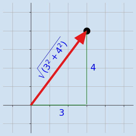
The two dimensions in 2D space are horizontal and vertical, which are perpendicular to each other. This can be used to calculate the length of a vector with the help of the Pythagorean theorem. The Pythagorean theorem states that, in a right-angled triangle, the square on the hypotenuse is equal to the sum of the squares of the other two sides.
In a right-angled triangle with sides of a and b and hypotenuse c then the
length of c is the square root of the sum of a-squared and b-squared.
$$ c = \sqrt{a^2 + b^2} $$
In the example the vector (3,4) below: $$ vector \ length = \sqrt{3^2 + 4^2} = \sqrt{9 + 16} = \sqrt{25} = 5 $$
 1(x, y) = (3, 4)
 2fig, [ax1, ax2] = plt.subplots(1, 2, figsize=(12, 8), facecolor=plt.cm.Blues(0.2))
 3fig.suptitle(
 4    f"Use Pythagorean theorem to calculate length of vector",
 5    fontsize=22,
 6    fontweight="bold",
 7)
 8
 9plot_axes(ax1, (x, y))
10ax1.set_title("Vector at point (3, 4)", fontsize=18, pad=20)
11ax1.annotate(
12    "",
13    (x, y),
14    xytext=(0, 0),
15    arrowprops=dict(ec=plt.cm.Set1(0), fc=plt.cm.Set1(0), headwidth=20, headlength=50),
16)
17
18plot_axes(ax2, (x, y))
19ax2.set_title("Right-angled triangle for vector (3,3)", fontsize=18, pad=20)
20ax2.annotate(
21    "", (x, y), xytext=(0, 0), arrowprops=dict(arrowstyle="-", ec="green", fc="green")
22)
23ax2.annotate(
24    "", (x, 0), xytext=(0, 0), arrowprops=dict(arrowstyle="-", ec="green", fc="green")
25)
26ax2.annotate(
27    "", (x, y), xytext=(x, 0), arrowprops=dict(arrowstyle="-", ec="green", fc="green")
28)
29ax2.tick_params(labelbottom=False)
30ax2.tick_params(labelleft=False)
31
32ax2.text(1.5, -0.2, "3", size=20, color="blue", ha="left", va="top")
33ax2.text(3.2, 2, "4", size=20, color="blue", ha="left", va="center")
34ax2.text(
35    1.3,
36    1.5,
37    r"$\sqrt{(3^2 + 4^2)}$",
38    size=20,
39    color="blue",
40    ha="center",
41    va="bottom",
42    rotation=50,
43)
44
45fig.tight_layout(pad=3.0)
46plt.show()

The length of a vector can be calculated in python with use of the Math functions module.
 1import math as m
 2
 3
 4def vector_length(v):
 5    return m.sqrt(v[0] ** 2 + v[1] ** 2)
 6
 7
 8for i in range(1, 6):
 9    v = (i, 4)
10    print(f"length of {v} is {vector_length(v):.1F}")
11
12"""
13length of (1, 4) is 4.1
14length of (2, 4) is 4.5
15length of (3, 4) is 5.0
16length of (4, 4) is 5.7
17length of (5, 4) is 6.4
18"""
Adding Vectors
Vectors can be added together by adding their individual constituent parts. In a way, this has already been done when considering a single vector like (3,4). This is composed of an x value of 3 and a y value of 4, which are vectors (3,0) and (0,4) and can be added to yield (3,4).
$$ (x_{1}, y_{1}) + (x_{2}, y_{2}) = (x_{1} + x_{2}, \ y_{1} + y_{2}) $$
The example shows the result of adding vector (3,4) to vector (-2, 1)
$$ (3, 4) + (-2, 1) = (3 + (-2), \ 4 + 1) = (1, 5) $$
 1(x1, y1) = (3, 4)
 2(x2, y2) = (-2, 1)
 3fig, axs = plt.subplots(1, 2, figsize=(12, 6), facecolor=plt.cm.Blues(0.2))
 4fig.suptitle(
 5    f"Adding two vectors",
 6    fontsize=22,
 7    fontweight="bold",
 8)
 9
10for a in axs:
11    a.set_facecolor(plt.cm.Blues(0.1))
12    a.plot(x1, y1, color="black", marker="o", markersize=15)
13    a.plot(x2, y2, color="black", marker="o", markersize=15)
14    a.spines["right"].set_visible(False)
15    a.spines["top"].set_visible(False)
16    a.spines["left"].set_position("zero")
17    a.spines["bottom"].set_position("zero")
18    a.set_xlim(-3.5, 4.5)
19    a.set_ylim(-0.5, 5.5)
20    a.grid(True)
21    a.tick_params(labelsize="large")
22
23axs[0].set_title(f"Vectors at point ({x1}, {y1}) and ({x2}, {y2})", fontsize=18, pad=20)
24axs[0].annotate(
25    "",
26    (x1, y1),
27    xytext=(0, 0),
28    arrowprops=dict(ec=plt.cm.Set1(0), fc=plt.cm.Set1(0), headwidth=20, headlength=50),
29)
30axs[0].annotate(
31    "",
32    (x2, y2),
33    xytext=(0, 0),
34    arrowprops=dict(ec=plt.cm.Set1(0), fc=plt.cm.Set1(0), headwidth=20, headlength=50),
35)
36
37
38axs[1].set_title(f"Sum of vectors = (1, 5)", fontsize=18, pad=20)
39axs[1].plot(x1 + x2, y1 + y2, color="black", marker="*", markersize=15)
40axs[1].annotate(
41    "",
42    (x1 + x2, y1 + y2),
43    xytext=(0, 0),
44    arrowprops=dict(ec=plt.cm.Set1(2), fc=plt.cm.Set1(2), headwidth=20, headlength=50),
45)
46axs[1].annotate(
47    "",
48    (x1, y1),
49    xytext=(0, 0),
50    arrowprops=dict(ls="--", arrowstyle="->", ec=plt.cm.Set1(0), fc=plt.cm.Set1(0)),
51)
52axs[1].annotate(
53    "",
54    (x2, y2),
55    xytext=(0, 0),
56    arrowprops=dict(ls="--", arrowstyle="->", ec=plt.cm.Set1(0), fc=plt.cm.Set1(0)),
57)
58axs[1].annotate(
59    "",
60    (x1 + x2, y1 + y2),
61    xytext=(x2, y2),
62    arrowprops=dict(ls="--", arrowstyle="->", ec=plt.cm.Set1(1), fc=plt.cm.Set1(1)),
63)
64axs[1].annotate(
65    "",
66    (x1 + x2, y1 + y2),
67    xytext=(x1, y1),
68    arrowprops=dict(ls="--", arrowstyle="->", ec=plt.cm.Set1(1), fc=plt.cm.Set1(1)),
69)
70
71
72fig.tight_layout(pad=3.0)
73plt.show()

Adding two vectors is the sum of the individual component parts
Addition can be extended to sum up any number of vectors by summing up their constituent parts. This can easily be performed in python by taking in a list of vectors and returning the resultant vector of the sum of the vectors.
 1def add_vectors(*v):
 2    return (sum([x[0] for x in v]), sum([x[1] for x in v]))
 3
 4
 5add_vectors((-2, 1), (3,4))
 6"""
 7(1, 5)
 8"""
 9
10add_vectors((1, 2), (0,6), (3,4))
11"""
12(4, 12)
13"""
14
15add_vectors((1, 2), (-5,-3), (3,4))
16"""
17(-1, 3)
18"""
Multiplying vectors by numbers
The addition of two identical vectors is equivalent to multiplying the vector by two. This can be extended to multiplying a vector by any number. Like addition, the resultant vector is got by multiplying the individual components by the number.
$$ (x, y) {\times} n = (x {\times} n, \ y {\times} n) $$
 1(x, y) = (3, 4)
 2fig, axs = plt.subplots(1, 2, figsize=(10, 7), facecolor=plt.cm.Blues(0.2))
 3fig.suptitle(
 4    f"Multiplying vector by a number",
 5    fontsize=22,
 6    fontweight="bold",
 7)
 8
 9for a in axs:
10    a.set_facecolor(plt.cm.Blues(0.1))
11    a.plot(x, y, color="black", marker="o", markersize=15)
12    a.spines["right"].set_visible(False)
13    a.spines["top"].set_visible(False)
14    a.spines["left"].set_position("zero")
15    a.spines["bottom"].set_position("zero")
16    a.set_xlim(-1.5, 13)
17    a.set_ylim(-2, 18)
18    a.set_aspect("equal")
19    a.grid(True)
20    a.set_xticks([x for x in range(0, 13, 2)])
21    a.set_yticks([x for x in range(0, 18, 2)])
22    a.tick_params(labelsize="medium")
23
24axs[0].set_title(f"Vector at point ({x}, {y})", fontsize=18, pad=20)
25axs[0].annotate(
26    "",
27    (x, y),
28    xytext=(0, 0),
29    arrowprops=dict(ec=plt.cm.Set1(0), fc=plt.cm.Set1(0), headwidth=25, headlength=30),
30)
31
32axs[1].set_title(f"Multiplication of vector by 2,3,4", fontsize=18, pad=20)
33for i in range(1, 5):
34    axs[1].plot(x * i, y * i, color="black", marker="*", markersize=15)
35    axs[1].annotate(
36        "",
37        (x * i, y * i),
38        xytext=(0, 0),
39        arrowprops=dict(
40            ec=plt.cm.Set1(0), alpha=0.2, fc=plt.cm.Set1(0), headwidth=25, headlength=30
41        ),
42    )
43
44fig.tight_layout(pad=3.0)
45plt.show()

A function can be created in python to multiply a vector by a number.
 1def multiply_vector(v, n):
 2    return (v[0] * n, v[1] * n)
 3
 4
 5for i in range(1, 6):
 6    print(f"vector (3,4) * {i} = {multiply_vector((3,4), i)}")
 7
 8"""
 9vector (3,4) * 1 = (3, 4)
10vector (3,4) * 2 = (6, 8)
11vector (3,4) * 3 = (9, 12)
12vector (3,4) * 4 = (12, 16)
13vector (3,4) * 5 = (15, 20)
14"""
Back to Pythagorean principle, it can be seen that scaling the vector (3,4) maintains the principle that the sum on the hypotenuse equals the sum of the squares on the other two sides. the famous triangle of 3,4,5 scales to other whole number combinations such as 6,8,10 or 15, 20, 25.
Table: vector (3,4) multiplied by factors showing the Pythagorean calculations
| Vector | factor | x-squared | y-Squared | sum | square root |
|---|---|---|---|---|---|
| (3, 4) | 1 | 9 | 16 | 25 | 5.0 |
| (6, 8) | 2 | 36 | 64 | 100 | 10.0 |
| (9, 12) | 3 | 81 | 144 | 225 | 15.0 |
| (12, 16) | 4 | 144 | 256 | 400 | 20.0 |
| (15, 20) | 5 | 225 | 400 | 625 | 25.0 |
Distance and Displacement
In geometry, Displacement is a vector whose length is the shortest distance from the initial to the final position of a point P undergoing motion. Displacement quantifies both the distance and direction along a straight line, whereas distance just measures the distance between two points without any direction.
The difference between two vectors is a displacement vector, although this includes the distance.
The displacement from (4,2) to (1,4) is (-3, 2)
$$ distance = \sqrt{-3^2 + 2^2} = \sqrt{9 + 4} = \sqrt{13} = 3.6 $$
 1(x1, y1) = (4, 2)
 2(x2, y2) = (1, 4)
 3fig, axs = plt.subplots(1, 2, figsize=(12, 6), facecolor=plt.cm.Blues(0.2))
 4fig.suptitle(
 5    f"Displacement from ({x1}, {y1}) to ({x2}, {y2}) is ({x2-x1}, {y2-y1})",
 6    fontsize=22,
 7    fontweight="bold",
 8)
 9
10for a in axs:
11    a.set_facecolor(plt.cm.Blues(0.1))
12    a.plot(x1, y1, color="black", marker="o", markersize=15)
13    a.plot(x2, y2, color="black", marker="o", markersize=15)
14    a.text(1, 4.3, f"({x2}, {y2})", size=16, color="blue", ha="center", va="bottom")
15    a.text(4, 2.4, f"({x1}, {y1})", size=16, color="blue", ha="center", va="bottom")
16    a.spines["right"].set_visible(False)
17    a.spines["top"].set_visible(False)
18    a.spines["left"].set_position("zero")
19    a.spines["bottom"].set_position("zero")
20    a.set_xlim(-3.5, 4.5)
21    a.set_ylim(-0.5, 5.5)
22    a.grid(True)
23    a.tick_params(labelsize="large")
24
25axs[0].set_title(f"Vectors ({x1}, {y1}) and ({x2}, {y2})", fontsize=18, pad=20)
26axs[0].annotate(
27    "",
28    (x1, y1),
29    xytext=(0, 0),
30    arrowprops=dict(ec=plt.cm.Set1(0), fc=plt.cm.Set1(0), headwidth=25, headlength=30),
31)
32axs[0].annotate(
33    "",
34    (x2, y2),
35    xytext=(0, 0),
36    arrowprops=dict(ec=plt.cm.Set1(0), fc=plt.cm.Set1(0), headwidth=25, headlength=30),
37)
38
39
40axs[1].set_title(f"Sum of vectors = (1, 5)", fontsize=18, pad=20)
41axs[1].plot(x2 - x1, y2 - y1, color="black", marker="*", markersize=15)
42axs[1].annotate(
43    "",
44    (x2 - x1, y2 - y1),
45    xytext=(0, 0),
46    arrowprops=dict(ec=plt.cm.Set1(1), fc=plt.cm.Set1(1), headwidth=25, headlength=30),
47)
48axs[1].annotate(
49    "",
50    (x1, y1),
51    xytext=(0, 0),
52    arrowprops=dict(ls="--", arrowstyle="->", ec=plt.cm.Set1(0), fc=plt.cm.Set1(0)),
53)
54axs[1].annotate(
55    "",
56    (x2, y2),
57    xytext=(0, 0),
58    arrowprops=dict(ls="--", arrowstyle="->", ec=plt.cm.Set1(0), fc=plt.cm.Set1(0)),
59)
60axs[1].annotate(
61    "",
62    (x2, y2),
63    xytext=(x1, y1),
64    arrowprops=dict(ec=plt.cm.Set1(1), fc=plt.cm.Set1(1), headwidth=25, headlength=30),
65)
66
67
68axs[1].text(
69    -1.1,
70    0.7,
71    f"({x2-x1}, {y2-y1})",
72    size=16,
73    color=plt.cm.Set1(1),
74    ha="center",
75    va="bottom",
76    rotation=-32,
77)
78axs[1].text(
79    2.9,
80    2.7,
81    f"({x2-x1}, {y2-y1})",
82    size=16,
83    color=plt.cm.Set1(1),
84    ha="center",
85    va="bottom",
86    rotation=-32,
87)
88
89fig.tight_layout(pad=3.0)
90plt.show()

Conclusion
This took me longer than I thought to write this article, but it has helped me learn more on Matplotlib and doing math with 2D vectors. The next article is still on 2 dimensional space with notes on segments, shapes, rotations and transformations.
matplotlib a comprehensive library for creating static, animated, and interactive visualizations in Python.
Math for Programmers by Paul Orland - a great book to brush up on your math skills.