Two Dimensional shapes

Jan 3, 2021 · 12 min read · python vector 2D mathplotlib ·

A vector has magnitude and direction. A single point in 2D space can be considered a vector from the origin (0,0) to that point. Vectors can be described anywhere in 2D space using a point for the start and a point for the end. Multiple vectors can be connected together to create 2D shapes. This article will discuss common 2D shapes as well as rotations and translations.

These are my notes on the book Math for Programmers by Paul Orland.

2D vectors and vector arithmetic
Two Dimensional shapes

Basic shapes

Simple shapes can be drawn by combining many vectors together. A square can be drawn using four points for the corners or four vectors for the sides. For vectors to draw shapes, one vector has to start where another vectors ends. previously, vectors were described as a single point where the origin (0,0) is the starting point. Vectors do not have to start at the origin and can be specified with a start point and end point

 1def plot_axes(ax, l_left, u_right):
 2    ax.set_facecolor(plt.cm.Blues(0.1))
 3
 4    # Hide the right and top spines
 5    ax.spines["right"].set_visible(False)
 6    ax.spines["top"].set_visible(False)
 7
 8    # Set the x and y axis to go through origin (0,0)
 9    ax.spines["left"].set_position("zero")
10    ax.spines["bottom"].set_position("zero")
11
12    ax.set_xlim(l_left[0], u_right[0])
13    ax.set_ylim(l_left[1], u_right[1])
14
15    ax.grid(True)
16
17    ax.tick_params(labelsize="medium")

 1def plot_segment(ax, v1, v2):
 2    ax.plot([v1[0], v2[0]], [v1[1], v2[1]], color="green")
 3
 4
 5fig, [ax1, ax2] = plt.subplots(1, 2, figsize=(9, 6.5), facecolor=plt.cm.Blues(0.2))
 6fig.suptitle(
 7    f"Basic Shapes",
 8    fontsize=22,
 9    fontweight="bold",
10)
11
12plot_axes(ax1, (-1, -1), (6, 6))
13ax1.set_title(f"Square", fontsize=14, pad=20)
14plot_segment(ax1, (1, 2), (4, 2))
15plot_segment(ax1, (1, 2), (1, 5))
16plot_segment(ax1, (4, 2), (4, 5))
17plot_segment(ax1, (1, 5), (4, 5))
18
19plot_axes(ax2, (-1, -1), (6, 6))
20ax2.set_title(f"Triangle", fontsize=14, pad=20)
21plot_segment(ax2, (1, 1), (4, 2))
22plot_segment(ax2, (1, 1), (2, 5))
23plot_segment(ax2, (4, 2), (2, 5))
24
25fig.tight_layout(pad=3.0)
26plt.show()
27
28publish_png_image(fig, "draw-square-triangle.png")

Draw a square and triangle

Polygon

A Polygon is a two-dimensional figure that is described by a finite number of straight line segments connected to form a closed shape. In the code above, there is a lot of repetition to create each segment of the shape. The following defines a mechanism of plotting a polygon based on a series of points. The last point is joined to the first point to close the shape.

1def plot_polygon(ax, *vertices):
2    # join the last vertex to the first to close the shape
3    vertices = vertices + (vertices[0],)
4    ax.plot([x[0] for x in vertices], [x[1] for x in vertices], color="red")

The same two shapes of square and triangle can be plotted using this function.

 1fig, [ax1, ax2] = plt.subplots(1, 2, figsize=(9, 6.5), facecolor=plt.cm.Blues(0.2))
 2fig.suptitle(
 3    f"Basic Shapes plotted as polygons",
 4    fontsize=22,
 5    fontweight="bold",
 6)
 7
 8plot_axes(ax1, (-1, -1), (6, 6))
 9ax1.set_title(f"Square", fontsize=14, pad=20)
10square = [(1, 2), (4, 2), (4, 5), (1, 5)]
11plot_polygon(ax1, *square)
12
13plot_axes(ax2, (-1, -1), (6, 6))
14ax2.set_title(f"Triangle", fontsize=14, pad=20)
15triangle = [(1, 1), (4, 2), (2, 5)]
16plot_polygon(ax2, *triangle)
17
18fig.tight_layout(pad=3.0)
19plt.show()

Draw a square and triangle with polygons

Plot complex polygons

A more complicated 2D shape can be plotted just by specifying a series of points in 2D-space. The following shows the code to plot an elephant.

 1fig, ax1 = plt.subplots(1, 1, figsize=(10, 9), facecolor=plt.cm.Blues(0.2))
 2fig.suptitle(
 3    f"More complex shapes",
 4    fontsize=22,
 5    fontweight="bold",
 6)
 7
 8plot_axes(ax1, (-15, -1), (16, 23))
 9ax1.set_title(f"Elephant", fontsize=14, pad=20)
10elephant = [
11    (2, 2),
12    (6, 2),
13    (6, 9),
14    (8, 12),
15    (9, 11),
16    (10, 7),
17    (12, 5),
18    (14, 6),
19    (15, 8),
20    (13, 8),
21    (12, 7.5),
22    (11, 9),
23    (11, 16),
24    (9, 20),
25    (4, 20),
26    (-6, 21),
27    (-10, 20),
28    (-13, 17),
29    (-13, 6),
30    (-12, 12),
31    (-11.5, 9),
32    (-12, 5),
33    (-11, 2),
34    (-8, 2),
35    (-9, 5),
36    (-8, 7),
37    (-8, 4),
38    (-7, 2),
39    (-4, 2),
40    (-5, 5),
41    (-4, 8),
42    (2, 8),
43]
44plot_polygon(ax1, *elephant)
45plt.show()

Plot an elephant polygons

Trigonometry and "sohcahtoa"

Trigonometry is the study of the relationships between side lengths and angles of triangles. In the previous article all vectors were described using x and y coordinates - this is the called the Cartesian coordinate system. A vector can also be described using the Polar coordinate, which consists of specifying the length (or magnitude) of the vector and the angle counter-clockwise from the horizontal.

To convert between Cartesian and Polar coordinates, we need to use the trigonometric rules from right-angled triangles. The rules can be remembered with use of the mnemonic SOHCAHTOA. The sine of an angle is equal to the length of the opposite side divided by the length of the hypotenuse (SOH); cosine equals adjacent over hypotenuse and tangent is equal to opposite over adjacent.

$$ sin θ = \frac {opposite} {hypotenuse} $$

$$ cos θ = \frac {adjacent} {hypotenuse} $$

$$ tan θ = \frac {opposite} {adjacent} $$

 1(x, y) = (3, 4)
 2fig, [ax1, ax2] = plt.subplots(1, 2, figsize=(9, 6.5), facecolor=plt.cm.Blues(0.2))
 3fig.suptitle(
 4    f"Trigonometry on a right-angled triangle",
 5    fontsize=22,
 6    fontweight="bold",
 7)
 8
 9plot_axes(ax1, (-1, -1), (4.5, 5.5))
10ax1.set_title(f"Vector at point ({x}, {y})", fontsize=14, pad=20)
11ax1.plot(x, y, color="black", marker="o", markersize=15)
12ax1.annotate(
13    "",
14    (x, y),
15    xytext=(0, 0),
16    arrowprops=dict(ec=plt.cm.Set1(0), fc=plt.cm.Set1(0), headwidth=25, headlength=30),
17)
18
19plot_axes(ax2, (-1, -1), (4.5, 5.5))
20ax2.set_title(f"Right-angled triangle for vector ({x}, {y})", fontsize=14, pad=20)
21ax2.plot(x, y, color="black", marker="o", markersize=15)
22ax2.annotate(
23    "", (x, y), xytext=(0, 0), arrowprops=dict(arrowstyle="-", ec="green", fc="green")
24)
25ax2.annotate(
26    "", (x, 0), xytext=(0, 0), arrowprops=dict(arrowstyle="-", ec="green", fc="green")
27)
28ax2.annotate(
29    "", (x, y), xytext=(x, 0), arrowprops=dict(arrowstyle="-", ec="green", fc="green")
30)
31ax2.annotate(
32    "",
33    (3.0, 0.5),
34    xytext=(2.5, 0),
35    arrowprops=dict(
36        arrowstyle="-",
37        color="blue",
38        connectionstyle="angle,angleA=-90,angleB=180,rad=0",
39    ),
40)
41
42
43ax2.tick_params(labelbottom=False)
44ax2.tick_params(labelleft=False)
45
46ax2.text(1.5, -0.2, "a", size=20, color="blue", ha="left", va="top")
47ax2.text(3.2, 2, "o", size=20, color="blue", ha="left", va="center")
48ax2.text(
49    1.5,
50    2.1,
51    r"h",
52    size=20,
53    color="blue",
54    ha="center",
55    va="bottom",
56    rotation=50,
57)
58ax2.annotate(
59    "",
60    (0.56, 0.8),
61    xytext=(0.85, 0),
62    arrowprops=dict(arrowstyle="-", color="blue", connectionstyle="arc3,rad=0.6"),
63)
64ax2.text(0.5, 0.1, "θ", size=20, color="blue", ha="left", va="bottom")
65
66fig.tight_layout(pad=3.0)
67plt.show()

Relationship between angles and line lengths in right-angled triangle

Relationship between angles and line lengths in a right-angled triangle

Conversion between Degrees and Radians

Angles in mathematics are often measured in Radian rather than in degrees. One radian being the angle formed with an arc the length of one radius. This means that 180 degrees is equal to π (pi) radians. Angles are generally given in degrees such as 15^o, 45^o, 90^o, etc.

$$ Angle \ in \ Radians = Angle \ in \ Degrees \times \frac {\pi} {180} $$

$$ Angle \ in \ Degrees = Angle \ in \ Radians \times \frac {180} {\pi} $$

sin, cos and tan are functions in the math module in python that take the angle in Radians. The inverse of these functions are asin, acos and atan also in the math module. These can be used to determine the angles in the right-angled triangle above with vector (3,4).

$$ sin θ = \frac {opposite} {hypotenuse} = \frac {4} {5} = 0.8 $$

sin θ = 0.8, using asin yields an angle of 0.927 radians.

$$ Angle \ in \ Degrees = Angle \ in \ Radians \times \frac {180} {\pi} = 0.927 \times \frac {180} {3.14} = 53.13^{\circ} $$

Validation of SOHCAHTOA
$$θ = 53.13^{\circ} = 0.927 \ Radians$$	$$sin \ 0.927 = 0.7998$$	$$\frac {opposite} {hypotenuse} = \frac {4} {5} = 0.8$$
$$θ = 53.13^{\circ} = 0.927 \ Radians$$	$$cos \ 0.927 = 0.600$$	$$\frac {adjacent} {hypotenuse} = \frac {3} {5} = 0.6$$
$$θ = 53.13^{\circ} = 0.927 \ Radians$$	$$tan \ 0.927 = 1.332$$	$$\frac {opposite} {adjacent} = \frac {4} {3} = 1.333$$

 1# vector of (3,4)
 2import math as m
 3angle = 4/5
 4"""
 50.8
 6"""
 7
 8m.asin(angle)
 9"""
100.9272952180016123
11"""
12
13m.asin(angle) * (180/m.pi)
14"""
1553.13010235415599
16"""
17
18m.sin(0.927), m.cos(0.927), m.tan(0.927)
19"""
200.7998228343401385 0.6002361482517589 1.3325136059694065
21"""
22
234/5, 3/5, 4/3
24"""
250.8 0.6 1.3333333333333333
26"""

Conversion between Cartesian and Polar coordinates

Cartesian coordinates specify a vector with an x-coordinate and a y-coordinate stating the horizontal and vertical distance from the origin. Polar coordinates specify the length (magnitude) of the vector and the angle from the horizontal axis.

There is a problem with relying on results of the inverse functions asin, acos and atan in that different coordinates may yield the same angle. Consider the vectors (3,4) and (-3,4) both have opposite length of 4 and hypotenuse length of 5. Multiple angles have the same sine, so the inverse sine gives one of these angles. It is possible to use inverse of all three functions to determine the exact angle, but the math module in python contains the function atan2 to get the correct angle based on vector coordinates.

 1help(m.atan2)
 2
 3"""
 4Help on built-in function atan2 in module math:
 5
 6atan2(y, x, /)
 7    Return the arc tangent (measured in radians) of y/x.
 8
 9    Unlike atan(y/x), the signs of both x and y are considered.
10"""

The following function makes use of math.atan2 to convert from Cartesian to Polar coordinates.

 1import math as m
 2
 3
 4def to_polar(v):
 5    angle = m.atan2(v[1], v[0])
 6    length = m.sqrt(v[0] ** 2 + v[1] ** 2)
 7    return (length, angle)
 8
 9
10print(to_polar((3, 4)))
11print(to_polar((-3, 4)))
12"""
13(5.0, 0.9272952180016122)
14(5.0, 2.214297435588181)
15"""

 1def to_cartesian(polar_v):
 2    return (polar_v[0] * m.cos(polar_v[1]), polar_v[0] * m.sin(polar_v[1]))
 3
 4
 5print(to_cartesian((5, 0.927)))
 6print(to_cartesian((5, 2.215)))
 7"""
 8(3.0011807412587945, 3.9991141717006924)
 9(-3.0028095170209874, 3.9978913197444705)
10"""

 1(x, y) = (3, 4)
 2fig, [ax1, ax2] = plt.subplots(1, 2, figsize=(9, 6), facecolor=plt.cm.Blues(0.2))
 3fig.suptitle(
 4    f"Cartesian and Polar coordinates",
 5    fontsize=22,
 6    fontweight="bold",
 7)
 8
 9plot_axes(ax1, (-1, -1), (4.5, 5.5))
10ax1.set_title(f"Cartesian coordinates", fontsize=14, pad=20)
11ax1.annotate(
12    "",
13    (x, y),
14    xytext=(0, 0),
15    arrowprops=dict(ec=plt.cm.Set1(0), fc=plt.cm.Set1(0), headwidth=25, headlength=30),
16)
17ax1.text(3.1, 4.3, "(3, 4)", size=20, color="blue", ha="center", va="center")
18
19
20plot_axes(ax2, (-1, -1), (4.5, 5.5))
21ax2.set_title(f"Polar coordinates", fontsize=14, pad=20)
22ax2.annotate(
23    "",
24    (x, y),
25    xytext=(0, 0),
26    arrowprops=dict(ec=plt.cm.Set1(0), fc=plt.cm.Set1(0), headwidth=25, headlength=30),
27)
28ax2.text(
29    1.4,
30    2.1,
31    r"5",
32    size=20,
33    color="blue",
34    ha="center",
35    va="bottom",
36    rotation=50,
37)
38ax2.annotate(
39    "",
40    (1.0, 1.3),
41    xytext=(1.6, 0),
42    arrowprops=dict(arrowstyle="<->", color="blue", connectionstyle="arc3,rad=0.4"),
43)
44ax2.text(0.4, 0.1, "0.927", size=20, color="blue", ha="left", va="bottom")
45
46fig.tight_layout(pad=1.0)
47plt.show()

Same vector described with Cartesian and Polar coordinates

Regular Polygons

A Regular polygon is a polygon where all angles are equal in measure and all sides have the same length. Polar coordinates can be used to quickly create a series of regular polygons, but it ie easier in Matplotlib to plot with Cartesian coordinates. These are regular polygons that fit inside a circle of radius 1.5.

 1def regular_polygon(n):
 2    return [to_cartesian((1.5, 2 * m.pi * x / n)) for x in range(0, n)]
 3
 4
 5fig, axs = plt.subplots(2, 4, figsize=(9, 6), facecolor=plt.cm.Blues(0.2))
 6fig.suptitle(
 7    f"Regular polygons",
 8    fontsize=22,
 9    fontweight="bold",
10)
11
12for i, ax in enumerate(axs.flatten()):
13    plot_axes(ax, (-2, -2), (2, 2))
14    ax.tick_params(labelbottom=False)
15    ax.tick_params(labelleft=False)
16    n = i + 3
17    ax.set_title(f"{n} sides", fontsize=14, pad=5)
18    p = regular_polygon(n)
19    plot_polygon(ax, *p)
20
21fig.tight_layout(pad=2.0)
22plt.show()

Regular polygons created with Polar coordinates and plotted with Cartesian coordinates

Rotation, Scaling and translation

Now that we have basic shapes, regular polygons and complex shapes, it is possible to plot the shapes, rotate the shapes, move or translate the shapes and/or change the size of (scale) the shapes. Translation moves every point of a shape by the same distance in a given direction. This can be achieved by adding the same (x,y) values to all coordinates of the shape. Rotate moves the shape around the origin by a specified angle, this is more easily done using polar coordinates. Scale is used to multiply each vector in a shape by a specified factor, a factor larger than 1 will increase the size of a shape and a factor less than 1 will decrease the size of the shape. The following functions are used to scale, transform and rotate and the plot_polygon function is updated to take a color as a parameter.

 1def plot_polygon(ax, color, *vertices):
 2    # join the last vertex to the first to close the shape
 3    vertices = vertices + (vertices[0],)
 4    ax.plot([x[0] for x in vertices], [x[1] for x in vertices], color=color)
 5
 6
 7def scale(n, v):
 8    return (n * v[0], n * v[1])
 9
10
11def translate(tran_v, vectors):
12    return [(tran_v[0] + v[0], tran_v[1] + v[1]) for v in vectors]
13
14
15def rotate(angle, vectors):
16    polar_vectors = [to_polar(v) for v in vectors]
17    return [to_cartesian((l, a + angle)) for l, a in polar_vectors]

 1elephant = [
 2    (2, 2),
 3    (6, 2),
 4    (6, 9),
 5    (8, 12),
 6    (9, 11),
 7    (10, 7),
 8    (12, 5),
 9    (14, 6),
10    (15, 8),
11    (13, 8),
12    (12, 7.5),
13    (11, 9),
14    (11, 16),
15    (9, 20),
16    (4, 20),
17    (-6, 21),
18    (-10, 20),
19    (-13, 17),
20    (-13, 6),
21    (-12, 12),
22    (-11.5, 9),
23    (-12, 5),
24    (-11, 2),
25    (-8, 2),
26    (-9, 5),
27    (-8, 7),
28    (-8, 4),
29    (-7, 2),
30    (-4, 2),
31    (-5, 5),
32    (-4, 8),
33    (2, 8),
34]
35
36fig, axs = plt.subplots(2, 2, figsize=(12, 8), facecolor=plt.cm.Blues(0.2))
37fig.suptitle(
38    f"Translate, Scale and Rotate shapes",
39    fontsize=22,
40    fontweight="bold",
41)
42
43titles = ["Elephant", "Scale", "Translate", "Rotate"]
44for i, ax in enumerate(axs.flatten()):
45    plot_axes(ax, (-20, -1), (30, 30))
46    ax.spines["bottom"].set_visible(False)
47    ax.spines["left"].set_visible(False)
48    n = i + 3
49    ax.set_title(f"{titles[i]}", fontsize=14, pad=5)
50    plot_polygon(ax, "red", *elephant)
51
52small_elephant = [scale(0.5, x) for x in elephant]
53plot_polygon(axs[0][1], "blue", *small_elephant)
54
55tran_elephant = translate((15, 6), elephant)
56plot_polygon(axs[1][0], "blue", *tran_elephant)
57
58rot_elephant = rotate(0.2, elephant)
59plot_polygon(axs[1][1], "blue", *rot_elephant)
60
61fig.tight_layout(pad=2.0)
62plt.show()

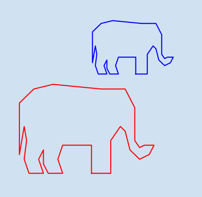
Scale, translate and rotate elephant shape

A variation of translation is reflection where the vectors of a shape are translated proportionally through a vertical line. Reflection through the maximum x coordinate is shown below to give the elephant a friend.

 1def vertical_reflection(vectors):
 2    # find max x value
 3    mir_x = max([x[0] for x in elephant])
 4    return [((-1 * (v[0] - mir_x)) + mir_x, v[1]) for v in vectors]
 5
 6
 7fig, ax = plt.subplots(1, 1, figsize=(10, 5), facecolor=plt.cm.Blues(0.2))
 8fig.suptitle(
 9    f"Reflection of a 2D shape",
10    fontsize=22,
11    fontweight="bold",
12)
13
14plot_axes(ax, (-20, -1), (50, 25))
15ax.spines["bottom"].set_visible(False)
16ax.spines["left"].set_visible(False)
17plot_polygon(ax, "red", *elephant)
18mirror_elephant = vertical_reflection(elephant)
19plot_polygon(ax, "blue", *mirror_elephant)
20
21fig.tight_layout(pad=2.0)
22plt.show()

Reflection of elephant shape

Conclusion

This article has completed the sections on 2D-space. Plotting basic and complex shapes using Matplotlib was detailed. A walk-through of trigonometric functions on a right-angled triangle and their use in converting between Polar and Cartesian coordinates. Once the initial shapes are plotted multiple versions of the shape can be generated using translation, rotation and scaling of vectors. Next article will start on 3 dimensional space and building on functions used in 2D-space.

matplotlib a comprehensive library for creating static, animated, and interactive visualizations in Python.

Math for Programmers by Paul Orland - a great book to brush up on your math skills.